Simulation Guide

Use magtrack.simulation to generate synthetic bead stacks and Z-LUTs for tutorials, benchmarking, or validating your analysis workflow. The examples below show the minimal inputs required to create stacks and capture both lateral and axial motion.

Quick start

Run the code block to generate a simulated bead:

import numpy as np
from magtrack.simulation import simulate_beads

# Define some motion (x, y, z in nanometers)
frames = 120
x_true = np.linspace(-150, 150, frames)
y_true = 80.0 * np.sin(np.linspace(0, 2 * np.pi, frames))
z_true = np.zeros_like(x_true)
xyz_true = np.column_stack([x_true, y_true, z_true])

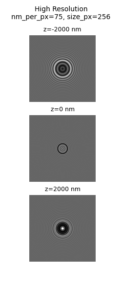
# Render a 256x256 pixel stack at 75 nm/px
stack = simulate_beads(xyz_true, size_px=256, nm_per_px=75.0)

# ``stack`` now has shape (256, 256, 120) and contains a single bead drifting and oscillating over time.

To visualize the bead, install matplotlib and run the code block below:

import matplotlib.pyplot as plt
plt.imshow(stack[:,:,0], cmap='gray')
plt.show()

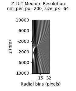
Run the code block to generate a simulated ZLUT:

import numpy as np
from magtrack.simulation import simulate_zlut

# Define some z-reference values (in nm)
z_min = -10000 # nm
z_step = 100   # nm
z_max = 10000  # nm
z_ref = np.arange(z_min, z_max+1, z_step)

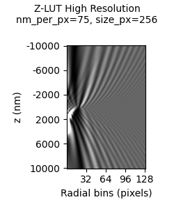
# Render a Z-LUT for beads with 256x256 pixel stack at 75 nm/px
# This generates a Z-LUT for profiles generated with radial_profile and oversample=1
zlut = simulate_zlut(z_ref, size_px=256, nm_per_px=75.0, oversample=1)

To visualize the bead, install matplotlib and run the code block below:

import matplotlib.pyplot as plt
plt.imshow(zlut[1:,:], cmap='gray')
plt.show()

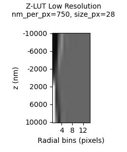
Tips for clean simulations

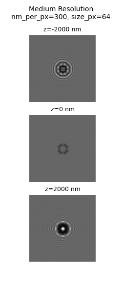
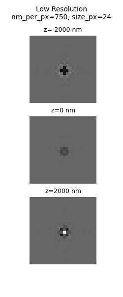
• Keep properties like nm_per_px consistent between simulations and downstream analysis to avoid scale mismatches.

• The simulation works best with larger image sizes (size_px >= 64px).

• The simulation is far from perfect. The wrong combination of parameters can create unrealistic images of beads. Start with the default simulation values and work your way towards what you want to simulate.

Examples