Benchmarking#
MagTrack ships with a small benchmarking harness that exercises each module in
benchmarks/ and records both CPU and GPU timings (when CuPy is installed).
The workflow is driven by benchmarks.run_all, which discovers every
callable whose name starts with benchmark_ and measures it with repeat
executions.
Running the orchestrator#
Launch the orchestrator directly from the project root:
python -m benchmarks.run_all
The command prints a short progress log while it imports benchmark modules and
runs their benchmark_* functions. CPU timings are always collected. GPU
measurements appear automatically when CuPy can access at least one CUDA
device.
System metadata and log layout#
Each invocation gathers host information so historical runs can be compared on
equal footing. The metadata includes the hostname, operating system, CPU and
memory (via psutil when available), GPU model details (via CuPy), the
Python implementation, and installed versions of magtrack, numpy,
scipy, and any distribution whose name contains cupy (for example,
cupy-cuda12x). The results are stored as JSON inside:
benchmarks/logs/<system-id>/<timestamp>/results.json
<system-id> combines the hostname, operating system, machine architecture,
and Python version. <timestamp> is a UTC time formatted as
YYYYMMDDTHHMMSSZ. These deterministic names make it easy to check the logs
into version control if desired.
Aggregated history#
After each run the orchestrator refreshes benchmarks/logs/combined_results.csv
with a flat table of every successful benchmark measurement. This CSV is
suitable for importing into pandas, spreadsheets, or other analysis tools. Use
it to look for long-term trends or regressions beyond the visual summary
produced by the plotting helper.
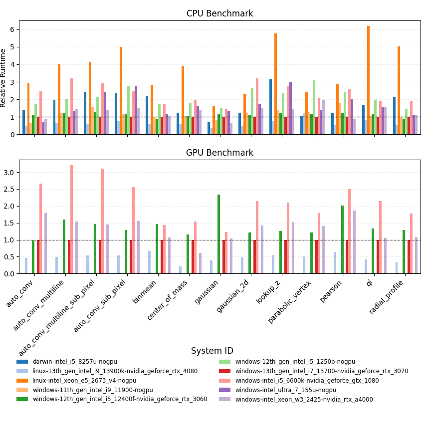
Interpreting the runtime plot#
Once the logs are written the orchestrator calls
benchmarks.plot_benchmarks.plot_benchmark_history(). The function loads
all historical entries, computes the average runtime for each
benchmark/backend pair, and then renders a grouped bar chart where every bar is
the average runtime recorded on a particular system. All values are plotted
relative to the cross-system mean so numbers above 1.0 indicate that a
machine typically runs that benchmark slower than the overall average, while
values below 1.0 are faster. The system that produced the most recent run
is highlighted with a bold outline, and a dashed horizontal line at 1.0
marks the long-term average so deviations stand out clearly. To make it easy to
spot how the latest execution compares against its host’s historical average,
an additional dashed outline overlays the exact measurements from the newest
run.
If Matplotlib is running in a non-interactive environment the figure object is
still returned, allowing you to save it manually (for example with
figure.savefig("latest_benchmarks.png")).
Publishing benchmark results#
MagTrack welcomes contributions that track performance trends over time. When you want to share a new set of logs, follow the same Git workflow you would for code changes:
Run the orchestrator and confirm the results appear under
benchmarks/logs/<system-id>/<timestamp>.Create a new branch and stage the generated artifacts:
git checkout -b benchmark/<short-description>
git add benchmarks/logs
Commit the changes with a message that summarizes the run, including any noteworthy hardware or software details:
git commit -m "Add benchmark results from <system-id> (<date>)"
Push your branch and open a pull request against
main. Publish the branch to your fork (or the upstream repository, if you have permission) with:git push -u origin benchmark/<short-description>
Then visit the repository on GitHub, click Compare & pull request, and target
main. In the PR body, mention the date of the run, the hardware you used, and any observations that might help reviewers interpret the numbers.
Following these steps keeps benchmarking history transparent and makes it easy for maintainers to review and merge performance data alongside code updates.